A Validity Map for the Gravitational Bohr Model - Reduced-Mass Algebra, Closed-Form Thresholds, and Applicability
The Core Idea
This notebook is about a very specific simplified universe: Newtonian gravity plus Bohr style quantized orbits. It does not claim new particles, new forces, or a new regime beyond known physics. What it offers instead is a carefully worked example of how a familiar idea runs into the limits of our existing theories, and how you can mark those limits clearly.
In that setting, the main result is a one page validity map. It shows where a hybrid Newton plus Bohr picture can be trusted, and where its assumptions must fail, forcing you back to classical interior gravity or forward to general relativity. The algebra that leads to that map is simple enough to do by hand, but it encodes a sharp lesson about domains of validity and scale.
Why I Started This
The project began with a question that felt almost too simple to ignore:
Can algebra alone tell you where the gravitational Bohr analogy stops being trustworthy?
Take two ingredients:
- Newtonian gravity for two masses \(M\) and \(m\)
- One basic quantum rule: allowed orbits come in discrete steps
From there, ask a straightforward question: How far can that picture go before it breaks, and which assumption fails first?
The Model Itself
The setup mirrors Bohr's old atomic picture but with gravity instead of electric charge. Two masses \(M\) and \(m\) orbit their common center of mass, and I treat it as a genuine two body system with reduced mass \[ \mu = \frac{M m}{M + m}. \]
In the standard point mass, nonrelativistic limit, the Newtonian orbit condition for relative motion is \[ \frac{\mu v^2}{r} = \frac{G M m}{r^2}, \] and the Bohr style quantization condition is \[ \mu v r = n \hbar \quad (n = 1, 2, 3, \ldots). \]
Combining these gives closed form expressions for the allowed orbits: \[ r_n = \frac{n^2 \hbar^2}{\mu G M m} \equiv n^2 a_g, \] where \[ a_g \equiv r_1 = \frac{\hbar^2}{\mu G M m} \] is the first allowed orbit radius. The corresponding energy levels are \[ E_n = - \frac{\mu (G M m)^2}{2 \hbar^2 n^2}. \]
These formulas are simple on purpose. They let you immediately compare the model to real physical length scales, without any numerical simulation. You can ask whether the first allowed orbit is outside the gravitating body, and how far it sits from the scale where strong gravity and relativity become important.
The Two Breakdowns
Once you have \(r_1\), two natural limits appear. Each one defines a guardrail on where the Newton plus Bohr construction can work.
Limit 1: finite size
The first breakdown is finite size. The Newtonian potential \( - G M m / r \) is a point mass idealization. It is not valid inside real matter, where the field depends on the mass distribution.
If the first allowed orbit lies inside the gravitating body, the model collapses immediately. In that case, interior gravity is the relevant physics, and the Bohr style orbit formulas no longer apply.
I model the body as a uniform density sphere with density \(\rho\), so its radius is \[ R_{\text{body}}(M) = \left( \frac{3 M}{4 \pi \rho} \right)^{1/3}. \]
The first guardrail is therefore the finite size condition \[ r_1(M, m) > R_{\text{body}}(M). \] If this inequality fails, we do not patch the model. We simply recognize that we have hit one of the limits of the point mass Newtonian picture and must replace that assumption.
Limit 2: strong gravity and relativity
The second breakdown is strong gravity. Even if the orbit lies outside the body, it can still sit so close to the relativistic scale that Newtonian gravity is no longer reliable.
The relevant scale here is the Schwarzschild radius \[ r_s(M) = \frac{2 G M}{c^2}. \] In the paper, I use a conservative weak field requirement: the first orbit should lie about one order of magnitude farther out than this radius, so that both the field and the orbital velocities are safely in the nonrelativistic regime.
This gives the strong gravity guardrail \[ r_1(M, m) \gtrsim 10\, r_s(M). \] If the first orbit approaches the Schwarzschild scale, then Newtonian gravity plus simple quantization is no longer a trustworthy combination, and a general relativistic treatment is required.
The Validity Window
These two conditions define a narrow window where the hybrid model is self consistent. Mathematically, the valid region is the set of points where both guardrails are satisfied:
\[ R_{\text{body}}(M) < r_1(M, m) \quad \text{and} \quad r_1(M, m) \gtrsim 10\, r_s(M). \]
When you plot these inequalities using the expressions for \(r_1(M, m)\), \(R_{\text{body}}(M)\), and \(r_s(M)\), you obtain an upper boundary from the finite size condition and a lower boundary from the strong gravity condition. The overlap between them is the validity window.
The figure below is a visual map of that overlap.
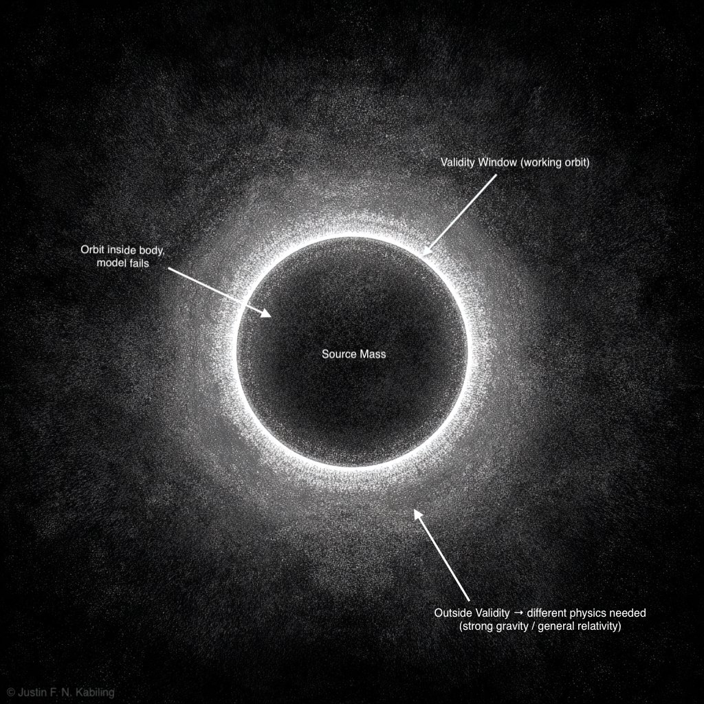

Reading the Map
The validity map is drawn in terms of source mass and orbital scale. One convenient choice is:
- Horizontal axis: mass \(M\) of the gravitating body
- Vertical axis: first allowed orbit radius \(r_1(M, m)\)
On this plot:
- The curve defined by \(r_1(M, m) = R_{\text{body}}(M)\) is the finite size guardrail. Above it, the first orbit lies outside the body. Below it, the orbit would sit inside the matter and the point mass picture fails.
- The curve defined by \(r_1(M, m) = 10\, r_s(M)\) is the strong gravity guardrail. Below it, the orbit is too close to the relativistic scale. Above it, gravity is still weak and Newtonian mechanics is reliable.
The valid region for the Newton plus Bohr construction is therefore the band in which the first orbit lies both outside the body and far from the strong gravity scale:
\[ R_{\text{body}}(M) < r_1(M, m) < \text{(finite size curve above)} \] and simultaneously \[ r_1(M, m) \gtrsim 10\, r_s(M). \]
On the map, this appears as a narrow window between the two guardrails. Outside that band, the picture is pushed either toward classical interior gravity (finite size breakdown) or toward general relativity (strong gravity breakdown), depending on which inequality fails first.
A Tangible Example
You can also plug in real numbers. A concrete case studied in the paper is a 1 kilogram laboratory mass binding a neutron. For that choice, \[ M = 1 \text{ kg}, \quad m = m_n, \] the first allowed orbit radius from the Bohr style formulas comes out to \[ r_1 \sim 10^{-5} \text{ m}, \] which is tens of micrometers.
That may sound surprisingly large, but it is still well inside any realistic 1 kilogram object, so the finite size condition fails immediately. Interior gravity is the relevant physics there, not the point mass potential, and the gravitational Bohr model is outside its domain of validity.
You can also look at the energy spacing. The levels satisfy \[ E_n = - \frac{\mu (G M m)^2}{2 \hbar^2 n^2}, \] so the spacing between the first two levels is \[ \Delta E_{1 \rightarrow 2} = E_2 - E_1, \quad \frac{\Delta E_{1 \rightarrow 2}}{h} \sim 1 \text{ Hz} \] for the neutron and 1 kilogram case. That is an extremely small scale, which explains why such hypothetical states would be very hard to observe even if the model were valid.
Interestingly, there are experiments that probe similar physics from a different angle. Ultracold neutrons bouncing above a mirror in Earth's gravitational field show quantization at comparable energy scales. They are not gravitational atoms in the Bohr sense, but they provide a real reference point near the same regime where the model's limits can be discussed.
The Bigger Lesson
Even in this very specialized construction, the outcome is general. A clean algebraic model has a domain where it works and clear boundaries where it does not. For the gravitational Bohr setup, Newtonian gravity plus quantized steps survives only inside a small window of mass and length scales. Outside that window, you are either forced back to classical interior gravity or pushed forward to general relativity.
More broadly, the map is a reminder that our theories are effective tools with borders, not final answers. The limits of physics in practice are the limits of these tools: where they apply, where they break, and how they hand off to the next framework.
What the validity map does is make that handoff visible on a single plot. It shows where a familiar semiclassical picture works, where it fails, and which assumption fails first. In that sense, the small gravitational Bohr model becomes a concrete way to talk about the limits of physics as we usually teach it, without claiming any new kind of atom or new fundamental regime. It is a diagram of consistency, drawn in the simplest algebraic setting I could find.